
This chapter discusses some of the basic skills required to get started with OxMetrics. The functionality of OxMetrics is the same under Linux, macOS, and Windows. The screen captures presented below were taken on Windows 10.
Since OxMetrics provides the data which other applications analyze, and receives all the text output and graphics which you create in (say) PcGive, you should begin by briefly learning how OxMetrics works.
Once OxMetrics has started, you will be able to load data, create graphs, and transform data using the OxMetrics calculator or algebra. Then, use the Model command on the Model menu to start econometric modelling using, for example, PcGive. When you exit OxMetrics it will automatically close all active applications which depend on it. In some of the coming tutorials we shall be using OxMetrics as a stand-alone program. There are many interesting things to be done even without using additional applications!
Start OxMetrics from the OxMetrics group on the Windows Start menu, or from a desktop icon.

If you install OxMetrics normally, it will already be registered, and you can start working immediately. An unregistered version will show the registration dialog on screen, as displayed above.
Enter the licensing code and your name in the respective fields (you must enter the code provided by the distributor).
An OxMetrics Enterprise licensing code enables most applications. Otherwise, many applications have their own additional licence code, which can be entered in the dialog. Once OxMetrics has the first registration code, the above dialog will not appear automatically anymore. To enter additional codes, activate the Help/Registration menu.
We trust that you use a legal copy of OxMetrics and client applications. That will allow us to keep developing the programs.
Without data, there is not much that can be done, so the first step is to load data. Many tutorials use a data set called data.oxdata.
The data file contions artificial data on consumption, income, inflation and output, denoted by CONS, INC, INFLAT, and OUTPUT respectively. OxMetrics can handle a wide range of data files, among them Excel files. You can also cut and paste data series directly from a spreadsheet (but not formulae).
We shall load this tutorial data set here. Access the File menu in OxMetrics, and choose Open. If you installed in the default directory structure, the data will be in the directory \Program Files\OxMetrics9\data, so locate that directory and select the data.oxdata file. (You will also see pairs of .in7/.bn7 files -- this was the default format in OxMetrics 8, and remains supported. In that case load the .in7 file.)
After loading, the data file becomes the currently active database for plotting and transformations. More than one database can be loaded, and the name of the currently active database is shown in the the toolbar. If more than one database is open, this toolbar box can be used to switch active database:

A notification of the loaded file is written to the Results window, so the loaded database does not acquire the focus. To see the database, click on it in the workspace. Although data values are stored internally with about 15 to 17 digit accuracy (8 byte floating point values), the data are displayed with 6 digits only in the spreadsheet:

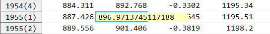
On the bottom right of the OxMetrics window, in the status bar, the observation under the cursor is shown with full accuracy:

Double clicking on the variable name shows the name and documentation of the variable, both of which can be changed. For the CONS variable:

The data can be manipulated, much like in a spreadsheet program. Pressing the left mouse button, and keeping it depressed, then dragging the mouse highlights a block of data which can be copied to the clipboard for insertion in another part of the database (click on the two-pages icon for copy, or the Ctrl+C key; paste is the clipboard icon or the Ctrl+V key).
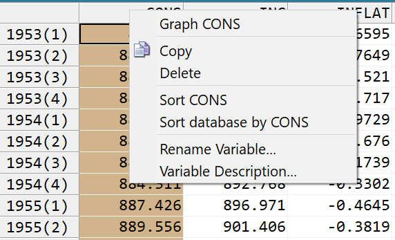
Right-clicking on the variable name brings up a context menu related to that variable, e.g. to quickly graph it. Here it is shown for CONS:
Two separate clicks will bring up the inline editor:
Right clicking shows the context menu. Select Edit Value to bring up a revision box, where corrected values can be entered (or missing values set to an observed outcome):

The graphics facilities of OxMetrics are powerful yet easy to use. This section will show you how to make time plots and scatter plots of variables in the database. OxMetrics offers automatic selections of scaling etc., but you will be able to edit these graphs, and change the default layout such as line colours and line types. Graphs can also be saved in a variety of formats for later use in a word processor, or for reloading into OxMetrics.
Graphics is the first entry on the Model menu. Alternatively, click on the graphics icon on the toolbar:

Either way brings up the following dialog box. This is an example of a dialog with a multiple selection list control. In such a list, you mark as many items as you want. Here we mark all the variables we wish to graph. With the keyboard, you can only mark a single variable (by using the arrow up and down keys), or range of variables (hold the shift key down while using the arrow up or down keys).
With the mouse there is more flexibility:

Here we select CONS and INC and then press the << button. This moves the variables from the database list to the selection list, activating the buttons at the bottom:

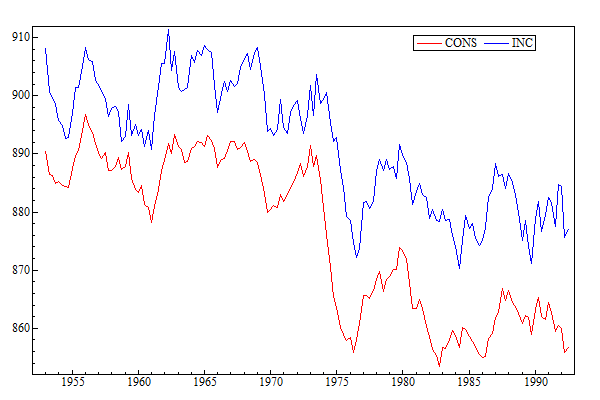
Press Actual series. Now the graph appears, which looks very much like Figure Figure:3.1. The only difference is the position of the legend. You can pick that up with the mouse, and move it to another position in the graph as desired.
Most graphs in this book are boxed in. You can change the default, for the current graph only, by double clicking on the graph (or selecting Edit/Edit Graph), then clicking on Graph layout in the left-hand column, and activating Box all areas, as shown here:

Alternatively, choose Graphics from the Model/Preferences menu, and activate Box all areas:

This will change the default for all future graphs that are made with OxMetrics.
Note that, when the graph is active, and the mouse is moved over the graph, the status bar at the foot of the OxMetrics window displays the graph coordinates. Inside a graph these are the `real-world coordinates' (X,Y), the actual data values. Outside these are `pixel coordinates' (pX,pY): a graphics window in OxMetrics runs from (0,0) in the bottom left, to (15000,10000) in the top right (further explanation is in Chapter ??).
One of the powerful features of OxMetrics is the ability to draw multiple graphs simultaneously on-screen within one graphics window (and you are not restricted to just one graphics window). We shall now get two graphs on screen, with the second a cross-plot of CONS and INC. Click on the Graphics toolbar button, note that CONS and INC are still selected (you can also variables to the opposing listbox by double clicking on them, or empty the selection by pressing Clear). The first variable in the selected list, CONS here, will be the Y variable (if CONS is not on top you can select it, and press the Move up button). Click on Scatter plot (YX) to create the plot.
If you accidentally did it wrong, click in the new sub plot (or plot area, as we tend to call it), selecting the entire second area, then press delete to remove it again.

A useful aspect of OxMetrics is that graphs can be edited and features added while they are on screen, and after adding other graphs if desired. Double click on the scatter plot graph, select Regression in the Edit Graphics dialog, and add one regression line as shown:

The final result is in Figure Figure:3.2. The editing possibilities are manifold: Chapter ?? provides a detailed discussion, but you can always play around with graphs at your leisure.
Finally, you can undo and redo the changes that were made. In this case, Undo will remove the graphics line again. Graph saving clears the undo/redo buffer, to avoid excessive memory use.
To print a graph directly to the printer when the graphics window has the focus, click on the printer icon in the toolbar. You can preview the result first using the Print Preview command from the File menu. If you have a PostScript printer, you can save the graph to disk as PostScript, and then print it from the command line.
Graphs can be saved to disk in various formats:
The GWG format is particular to OxMetrics; no other program can read it and no printer can handle it. OxMetrics requires the GWG format, because it needs to be able to allow re-editing of the graph when it is reloaded; the other formats do not store sufficient information. When you save a graph in any format, the GWG file is automatically saved alongside it. Then, when loading a previously saved PDF file (say), OxMetrics can use the GWG file to reload the graph.
There is an important distinction between copying graphs for use in internal OxMetrics graphs, or for external use.
To paste the graph into Word, for example,
you can use Edit/Copy Metafile to Clipboard, and then
paste it into Word. A metafile stores the actual Windows commands
that were used to draw the graph, and thus scales well. The
alternative is to copy the bitmap to the clipboard.
The standard copy command is used for internal paste. If no area is selected, the whole graph is copied, otherwise the selected area only.
Try this by clicking on the second area in the current graph. Once selected (shown by a hatched boundary) copy the area to the clipboard. Then first deselect the area by clicking somewhere in the margin of the graph. A subsequent paste will add a copy as the third area. Next, select the first area and paste again: this inserts the cross-plot into the time-series plot (not a useful graph).
Two options are available for transforming data: by algebra or by a dialog approach, which mimics the operation of a pocket calculator. We begin with the latter, as it is the simplest.
Please note that OxMetrics and client applications are sensitive to the case of the variable names so that `cons', `Cons', and `CONS' are treated as different variables. This can be useful for distinguishing real (lower case) from nominal (capitals) variables, or logs from levels, etc.
In several cases OxMetrics will offer a default name for a newly created variable:
So can you guess what DLCONS_1 is likely to be?
The aim is to build up an algebraic expression for the transformation (which is valid Algebra code: see §3.5). Press on the Calculator button leading to the capture shown below (or via the Model menu and Calculator choice).

The first transformation is to take the first difference of CONS. Click on the CONS variable just to highlight it (don't double click), and then on the diff button, accept a lag length of one, to see in the top part of the dialog:

Click on the large button with the = sign, and accept the default name of DCONS, which will be created in the database, and added to the list of variables. A two-period difference is just as easy to compute: select CONS, press the diff button and change the length of the differencing period.
Another transformation to try: INC-CONS. Double click on INC, click on the minus button, and then double click on CONS. The expression now reads INC--CONS, press on = to evaluate. Name the variable SAVING (you could use a name like INC--CONS, but must enclose such a name in double quotes when using it in expressions).
Finally, we create a step dummy (or indicator variable), where the step lasts from 1979(2) to 1980(4). We need zeros outside that period, ones inside. Click on the dummy button, and enter:

Click on OK, and then on = to create the dummy. Give it an informative name, such as s792t804.
Three additional operations can be performed on variables inside the listbox in the Calculator:
All changes to the database can be undone from the Edit menu.
Exit the calculator (Esc or click on the x button), and graph some of the variables to check whether the transformations are correct. All transformations are logged to the Results window:
    Algebra code for data.oxdata:
    DCONS = diff(CONS,1);
    SAVING = INC-CONS;
    s792t804 = dummy(1979,2, 1980,4);
This leads us to the next topic.
Algebra enables us to do transformations by typing the expressions directly into an editor. It also allows saving and loading from disk of a whole chunk of statements.
As an example, we rerun the transformations of the previous section. To verify if that will work, activate the database, and press Undo until the database is back in its original state. Now set focus to the Results window. Locate the logged Algebra code in the Results window. There are two ways to quickly run this code:
Because the former is straightforward, we now discuss the latter method.
Highlight the three algebra lines, and copy them to the clipboard (Ctrl+C). From the Model menu, select Algebra, and paste the code (Ctrl+V) to see:
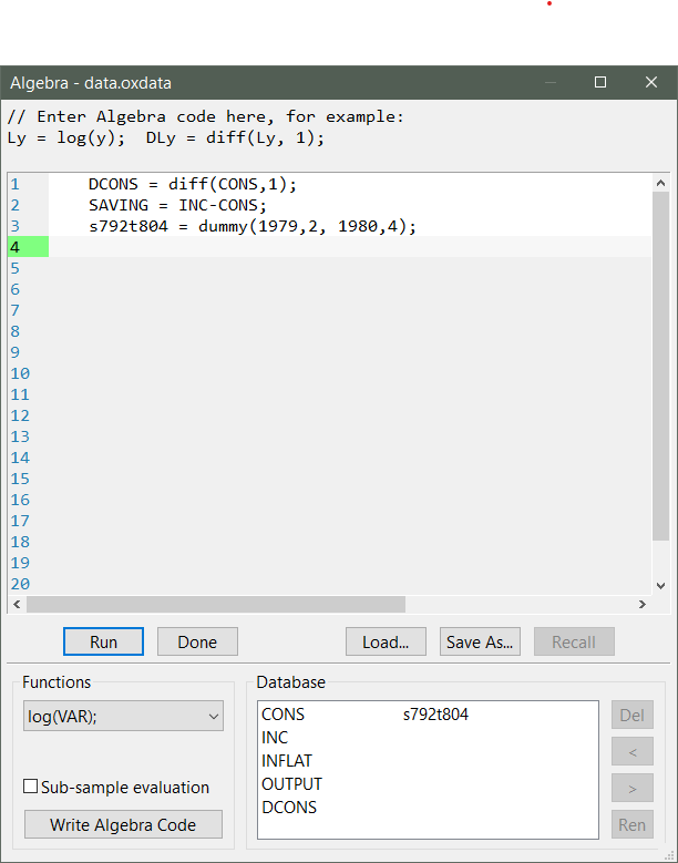
Now press Run. The variables have been recreated. We can inspect the database to see what happened. The algebra code is again logged to the Results window.
The only variable names allowed directly in Algebra are those that would be valid names in computer languages like Ox or C: the first character must be a letter or an underscore, the rest a letter, underscore or digit. Names which do not follow this convention may be used as well, but must be enclosed in double quotes.
Algebra uses database variables as follows: if a left-hand variable is already in the database it will be overwritten, otherwise it will be created. Variables on the right must exist, possibly because of preceding lines of algebra code. Algebra is case-sensitive, meaning that LCONS, LCons and lcons refer to three different variables.
An impulse indicator for 1980(1) can be created as
The same dummy can also be created using the insample function and a conditional assignment. The insample function has four arguments: startyear, startperiod, endyear, endperiod. It returns 1 (or TRUE: everything which is not 0 is TRUE) if the observation under consideration falls within the sample, otherwise it returns 0 (FALSE). The conditional assignment works as follows: the conditional statement (the `if' part) is followed by a question mark and the `then' part, which is followed by a colon and the `else' part. Read:
An error message pops up if you make a mistake. The error can be corrected on returning to the algebra editor. The text at the top of the Algebra error shows the text of the last error (if one occurred).
Do not save the modified data set. Either undo the changes, or quit the data set, and reload the original data.oxdata. Algebra is documented in Chapter ??.
This completes the getting-started chapter. Before giving some examples on modelling with OxMetrics, we briefly discuss the workspace window. The remainder of the tutorial are more detailed examples on graph editing, graphics, data loading and saving, and data transformations.
Often, after working in OxMetrics for a while, there are many open documents, with graphs, data and results. The workspace on the left helps navigating between these, by showing which documents are open in OxMetrics.
An example is shown at the start of this chapter. Here there are two data files open (if a document has been modified it indicated by the * in front of the name). There is one graph, a code file simnor.ox, and the finally the Results window. The available apps are listed under Applications (with all interactive modelling packages such as PcGive, STAMP, etc. now grouped under the Model header).
Right clicking on the document category (Data, Graphics, Code, or Text) gives a context menu. For Data it is:

while right clicking on the document name gives:
General settings are controlled from the Preferences dialog:

For Windows and Linux this allows a switch to dark mode (requiring a restart of OxMetrics). Under macOS dark mode is set in the operating system. It also allows for a change of the default fixed width font and size. But the text size can also be controlled directly from the View menu.
Chapter 4, which is the next in line, introduces the OxMetrics applications. This includes an example on estimating a GARCH(1,1) model using PcGive. Because OxMetrics behaves very similarly on Windows, OS X and Linux, we shall not explicitly distinguish between the different platforms in the remainder.
There is an increasing number of computer programs which cooperate with OxMetrics to deliver an easy-to-use yet powerful user experience. Such applications implement different services, and may use OxMetrics:
At the time of writing, the OxMetrics compatible applications accessed via the Model command include:
Further applications include:
In addition, there are interactive packages written in Ox which can be run via OxPack.
It is possible that only a subset of the applications are installed. The remainder of this chapter gives a brief introduction on how to use PcGive. Even if PcGive is not one of the applications you plan to use, it will still be useful to read it: most applications work in a similar way. Before we start, we load another database, and digress by talking about financial data.
Load the dowjones.xlsx data set from the OxMetrics9\data
folder.
The DOWJONES variable holds the weekly Dow--Jones index
(Dow Jones Industrial Average): close at midweek
from Janary 1980 to September 1994, 770 observations in total.
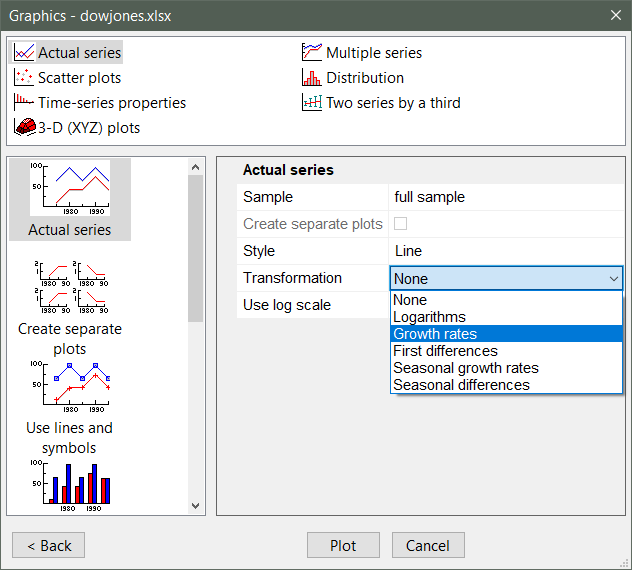
We are interested in the returns, log Yt- log Yt-1, already in the database as DLDOWJONES. First, we illustrate the the returns can also be plotted directly from the levels. Make sure dowjones.xlsx is the active database. Click on Graphics, select DOWJONES, and click on All plot types>. Then select transformation Growth rates:
The outcomes are given in the top panel of Figure Figure:4.1. The large negative return of -17.4% corresponds to the Black Monday crash of 19 October 1987. The data show behaviour that is typical of financial time-series: clustering of volatility and so-called thick tails: there are more observations in the tail than can be expected from a normal distribution.
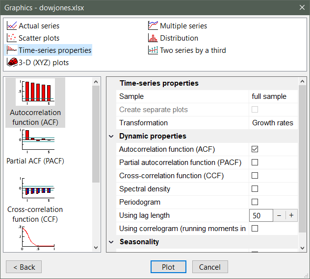
Next, activate Graphics again, using the same variable. Select time-series properties and note that the transformation is still set to growth rates. Click on ACF, and set the lag length to 50:
The outcomes are in the second panel of top panel of Figure Figure:4.1, indicating that there does not seem to be much memory, if any, in the returns. This should be expected. Next, use the calculator, and create the squared returns. The ACF of the squared returns are in the final panel of Figure Figure:4.1 (remember to reset the transformation back to none). This plot suggests that there is indeed some persistence in volatility.

When moving the cursor over the graph of the actual returns, the status bar at the bottom can be seen to display the date in the plot. There are too many observations for an accurate reading, but the large negative shock can be pinpointed in October 1987.
Inspection of the database reveals that the first variable is called Date, and shows the same dates as in the row labels:

Double-clicking on the variable name reveals that it is of type Date. Changing it to Default changes the labelling to an undated dataset, and the Date values to large numbers:

These are the numbers that OxMetrics and Ox use to represent dates. Any fractional value represents fractional time (so 0.5 is 12:00 and 0.75 18:00 on the 24-hour clock).
Undo the changes to get back to the dated database. With weekly data, there are some years that have 52 weeks, and others with 53. Therefore, the method of using a fixed frequency, as used for annual, quarterly and monthly databases, does not work. Instead, a database can now be dated:
These criteria are satisfied in dowjones.xlsx, and the Excel dates are translated in Ox dates when reading the file (and the other way round when saving). Database!--- with dates
Next, to illustrate the modelling sequence in OxMetrics, we estimate a GARCH model without paying too much attention to the actual outcomes.
PcGive is an interactive program for dynamic econometric modelling. Like other interactive modelling packages, it can be started in three ways:


The modelling dialog gives access to all the modelling features of the OxMetrics applications. In this case, only STAMP and PcGive are listed, but you may have more. The application will use one of the databases loaded in OxMetrics.
The first step is to select a model category, and for the category a model type. The images at the top allow you to see the choices for all available applications, or to restrict it to a specific application. In your case, it is likely that Module is set to all (if not, click on the OxMetrics item for All, or on PcGive).
Change the Category to financial data and the model to GARCH.


Click on the large Formulate button, to see the standard formulation dialog. On the right-hand side is the list with the database content, while the box on the left, empty as yet, is for the model.
This dialog is used by most applications to formulate the linear part of the model. Other actions that can be taken are:
For the GARCH model there are three types:
If another status is selected in the drop down box, that will be used for the added variables instead of the default (but lagged variables can never be the dependent variable).
To change status of variables that are already in the model: highlight the variables in the selection box, choose a status, and press the Set button. Note that it is also possible to change status by right-clicking on a variable.
Double click on the DLDOWJONES variable:

Press on Next to set the GARCH model properties. There are quite a few options, but the default of a GARCH(1,1) model suffices:

The final step is the estimation period, where we can accept the default again:
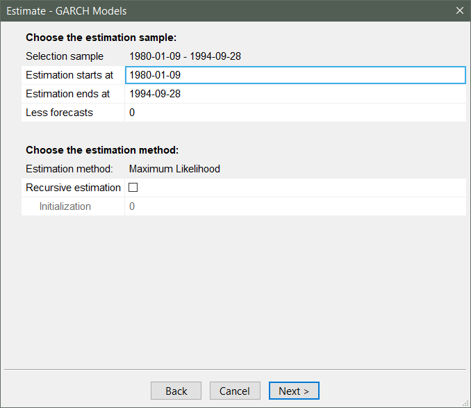
Click on OK and the output appears in the results window.
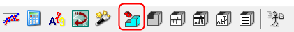
To end this section, consider all the buttons available for modelling:

They are respectively:
Graphic Analysis is available from the toolbar button as well as the Test menu button. To see this, click on the latter:

and accept the default choice. The figure is as in Figure Figure:4.2. Note that in the middle panel (the standardized residuals), we zoomed in on the crash and changed the style to index lines. It is quite likely that this large outlier affects the quality of this model (, and , ).
